This is a transcript of a talk delivered at the Bartlett school of Architecture on March 24th 2010, as part of a series of seminars held by the Center for Advanced Spatial Analysis (CASA) at University College London. This is my first academic seminar, in which I lay out some of my research aims and their conceptual underpinnnings. You can see the original presentation in the format it was delivered here.

Hello. My talk is called microplexes.

It’s a presentation on how very small complex systems can show us how to grow large urban systems.

Today I want to talk about scale. It strikes me that modern knowledge is intensely specialised by scale.

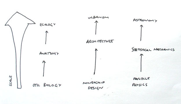
This is one of the first sketches I put in my notebook when I started my PhD 6 months ago. It seemed a bit throwaway to me at the time, and of course it isn’t very accurate in how it links disciplines, but its core message of scales of knowledge holds I think. I’m trying to work in a cross-scalar manner in my own research.

I want to show you how network topologies give us a means of analysing and comparing spatial systems at disparate scales, how network science gives us a vocabulary for talking about any spatial system and what the limitations of that vocabulary might be.

The cell biologist and the ecologist will tell you that they work in different fields of the same branch of knowledge, invoking the kind of tree taxonomy of knowledge sketched by Diderot in the 18th Century.

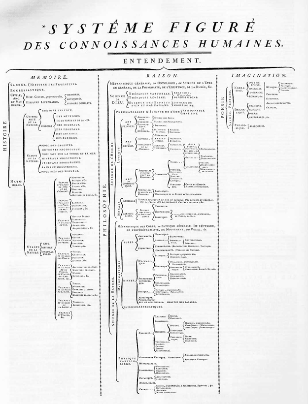
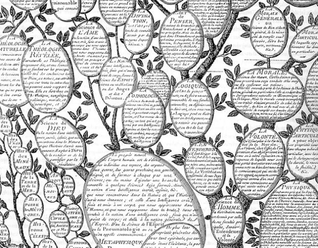
Fields and branches are, of course, metaphors borrowed from nature. Here’s another attempt from Diderot to construct a ‘figurative’ system of knowledge, an information visualisation of knowledge structures.

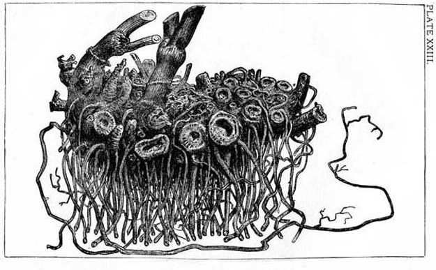
Keeping to this tradition of biological metaphor I see knowledge, like the french philosopher Gilles Deleuze, better thought of in terms of rhizomes. The potato is a rhizome. A rhizome is a tubular root which has a non-hierarchical, decentralised structure of tubers, shoots and stems. It can give rise to many inputs and outputs, spawning new growths in multiple locations. The picture you are looking at is that of a rhizome.

Of course, networks can be non-hierarchical, and, depending on the rules of engagement, nodes can accommodate many inputs and outputs, so we can think of knowledge, or the rhizome, as a particular type of network. Since we live in a network society, it is intuitive to us that knowledge is both intensely horizontally networked as well as arborescent, clustered as well as cascading, and that there is a dichotomy between these two topologies, the mesh and the tree.

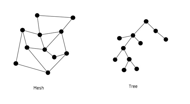
one highly decentralised and the other highly hierarchical. I will try to show how this interplay exists in many complex networks, not just our systems of knowledge.

Very different topologies often exist at different scales of a complex network. A principle assertion of mine is that complex systems are characterised by scales of connectivity, we can see this by looking at the rhizome structure itself. At its top-level, its topology looks a bit like this.

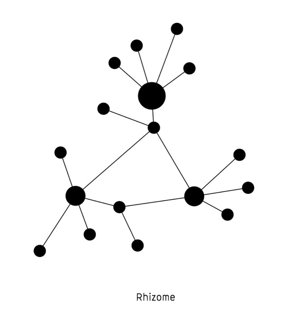
A mixture of the dendritic structure associated with tree topologies and a meshwork. But if we take a microscope to a shoot in the rhizome it’ll look a little like this.

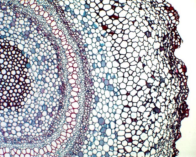
Here we see a vascular bundle of cells, a dense packing forming concentric circles, we see deformations produced by contractile forces and gradients. We see an optimisation of surface area between cell membranes as well as a large diversity of passages between cells, a morphology optimised for two transport scenarios – one to permit the diffusion of material through cell membranes via osmosis and another to allow materials to percolate through the system between the cell boundaries, a highly porous structure. The xylem and phloem cells in this fern rhizome we’re looking at allow water and sugars to permeate the cell tissue and travel down the rhizome stem via diffusion induced by gradients.

Importantly, if we look at the topology of this cellular structure, we see that each cell is only interconnected with its closest neighbours, there are no long range connections in this system. If we model each cell as a node, and contact with other cells as a link, the topology looks a bit like this.

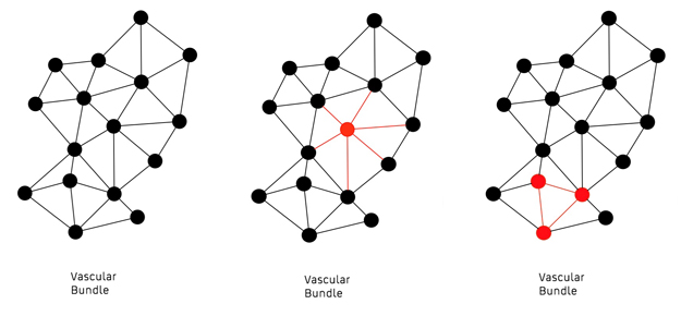
To a mathematician it looks like a Delaunay triangulation. There are no hubs, and there is no dendritic system, there is no tree, just a meshwork. We say there is a narrow distribution of degrees of connectivity, where a node’s degree denotes the number of other nodes it is linked to. The distribution here is based on cell size and the radius of the vascular bundle at which the cell happens to be. We call this a highly clustered topology because it’s full of linked triplets of nodes, this property is known as triadic closure and was discovered in social networks.

Decentralised mesh topologies, gradients and high clustering appear to be characteristic of self-assembling, self-organising complex systems, of which more later.

So even in a rhizome itself, Deleuze’s proposed metaphor for the structure of knowledge, we can see how scales of connectivity are characteristic of complex systems. It’s just that in the case of the rhizome, the structure is sufficiently complex that we need a microscope to make this apparent.

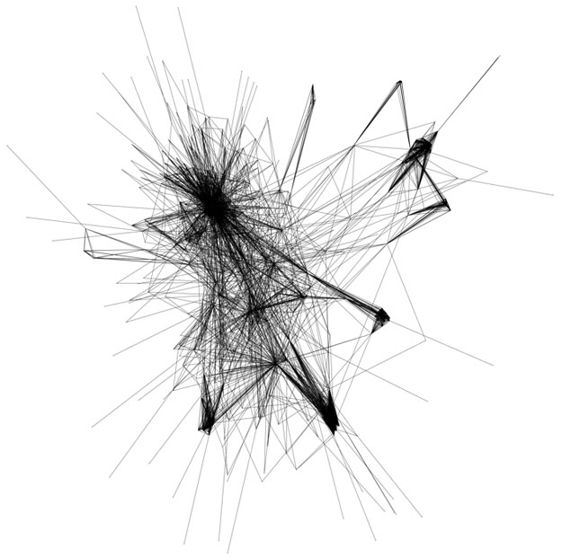
My comments on the rhizome aren’t entirely speculation. We have some insight as to knowledge structure through the analysis of document linkage in wikipedia. Here’s a small subgraph rendered by Ian Pearce showing connectivity in a few thousand wikipedia pages. You can see straight away both hubs and dense clustering, the interplay of star and mesh topologies.

Rosvall & Bergstrom rendered this directed, weighted graph visualising an online citation network between several thousand academic papers. The volume of citations is expressed in link widths and colours, the size of the nodes communicates the amount of time spent surfing papers in that topic by readers. In this analysis they found hierarchies of topics, with many flows from the applied sciences directed at a smaller set of natural sciences. These natural sciences in turn form a ring-like topology of citations between themselves.

So in these knowledge networks we see different topologies at different scales, we see scales of connectivity.

Through these examples I seek to show how networks give us a toolkit to skip between these disparate systems, both spatial and virtual, systems as diverse as human knowledge and a tiny vascular bundle of cells.

I’d like to look now at some microscopic spatial systems. Let’s begin with a human artefact which I consider to be the smallest example of organised complexity in what we call the built landscape: the microchip.

Microchips

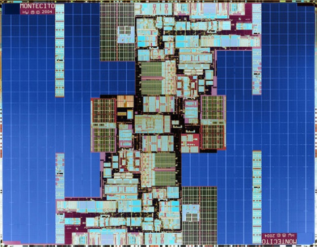
This is Montecito, Intel’s dual core chip from 2006, with 1.7 billion transistors fused onto a silicon substrate about 2×2cm in dimensions. The surface area of Montecito is smaller than that of a £2 coin. Let’s look at the spatial logic of this chip. You can tell it’s dual core because it essentially contains a mirror image around a horizontal axis.

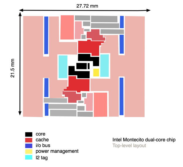
As you can see a microchip is essentially an agglomeration of memory, coloured in red, around a small core of central processing units, which are coloured in black. Memory comes in the form of caches. There are about four-levels of caches in Montecito, the more intense the colouring, the speedier the cache access. These are low activity areas designed simply to store data in between instructions. Along both sides you see a sprawl of low-speed memory. The whole chip is bounded by an interface to the rest of the hardware in the form of an I/O Bus. A Bus describes a particular type of network topology in which one central link serves to transport information across a lot of nodes. Note that power management is a compact unit just off center, coloured in yellow here.

The components in a microchip are synchronised using a clock subsystem and signal dynamics are strictly sequential within a single core. The chip is optimised for round trips between the caches and the core, as these occur multiple times during the most rudimentary of instructions. Current travels between these components on the scale of nano seconds.

Microchips are laid out in this configuration using multiple phases of heuristic design. Floorplanning, packing and optimisation algorithms create this top-level structure as well as the lower level configurations. Microchip designers model the chip as a network, grouping the billions of components into just hundreds of logical units by identifying where clustering levels are high. The top-level topology of a microchip is centered around a small number of core components but at lower levels, it can look like a highly clustered graph. Again we see scales of connectivity here.

So in a microchip we see an intense logic of integration, as evidenced by its name, the integrated circuit. In this case, optimisation of connectivity lengths, energy consumption and the spatial footprint of components is carried out algorithmically. The microchip is an example of high levels of integration and density creating high energy efficiency in a complex signal processing system. I would say the spatial outcome is one of organised complexity, organised that is, by microchip designers acting as a centralised agency. In this sense, they can be considered master-planners of a static, non-living system.

Here is an example of what a microchip city might look like if you planned an urban system in the image of a micro-processor.

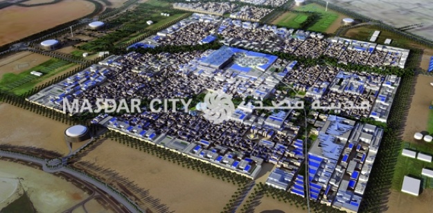
This master-plan, Masdar, was proposed by Foster & Partners in Abu Dhabi. It’s a high-density, compact, highly interlinked, walkable urbanisation of 50,000 revolving around a business core. Foster & Partners explicitly state the microchip as design inspiration for the project. It’s no surprise to see the microchip invoked in such a way. After all, our cities too have grown as agglomerations around cores. They too have become polycentric, or multicore, over time, in order to become more efficient processors of their own. They too have optimised transport to and from their cores, where the vast majority of their activity takes place. They too contain multiple levels of low activity bands in the form of residential zones. However imperfect the analogy, it is safe to say that we see a number of echoes of urban morphology in this microscopic human artefact, and that in both we see the effects of organised complexity.

Now let’s look at another information processing network with components on a similar scale, but with a self-organising dynamic, the neural network that describes our brain.

Neural Networks

A human neuron and a transistor on average have dimensions of about 1 micron, or 10^-6 meters, but a brain contains an order of magnitude more neurons than contemporary microchips possess transistors, about 10 billion. Note that the neuron is significantly more complex in topology than a transistor, which can be considered simply as a switch.

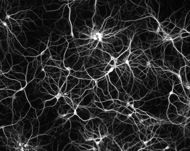
Both the adult human brain and Montecito consume about the same energy, 100 watts, but they are radically different in terms of processing and topology. The brain is a massively parallelised, decentralised processing architecture. It’s often very highly clustered. It’s normal for a neuron to have around 10,000 synaptic links to other neurons in a human brain, whereas a transistor or logic gate rarely takes more than 3 inputs. This disparity in degree distribution and clustering properties highlights the core differences between these two information processing networks.

A brain then, is analogous not to a microchip, which is serialised and centralised, but to a large network of microchips, something like the World Wide Web, another self-organised system. By using network representations we can make these comparisons across vast spatial scales in a quantitative manner. We can say that both the brain and the internet display scale-free degree properties as well as connectivity features reminiscent of small-world networks. Let’s look at this latter feature.

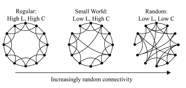
A small-world network exhibits low mean path lengths between any two arbitary nodes (L on the diagram) and yet contains high clustering coefficients (C on the diagram). You can see here that it is characterised by lots of local connectivity between nodes, as well as the occasional longer link, a shortcut if you will. Only a few of these longer links are required in order to tip the network, in what is known as a phase transition, from a relatively poorly connected global state into a small-world state. From a spatial network standpoint, small worlds mean high levels of mean accessibility from any given node to any other node, a homogenous distribution of high levels of mobility if you will. We see small-world properties primarily in self-organised networks. They were first observed in social networks by Watts & Strogatz.

Coming back to neural networks. If we look at the growth of the brain, or neurogenesis, we see that it is both a self-assembling structure, as neurons and dendrites grow and reproduce, and a self-organising structure, as neurons determine which other neurons to connect to, each neuron developing its dendrites, probing into its surroundings in search of neighbouring neurons and forming new synapses.

Let’s look more closely at this mechanism of biological growth.

Morphogenesis

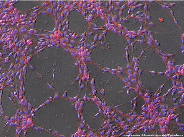
Here we can see epithelial cells in a collagen substrate doing a similar thing to neurons; spontaneously forming networks via random motion and outreach.

The networks they produce via this mechanism are strongly meshlike in topology. This kind of self-organised network formation is not often seen in urban growth as it requires the unsupervised growth of self-interested agents, or nodes. I will allow myself to speculate that you may see it in the development of linkages between urban centers that proliferate over a long period of time, particularly where regional policies relating to compactness or urban containment are not present.

The probing we see here due to cell tip growth is a form of morphogenesis. The term morphogenesis describes the various processes that result in the development of form in cellular biological systems. Let’s look at more morphogenetic processes, because they can show us some spatial outcomes of self-organisation.

Here’s one of the most fundamental, mitosis,

It is interesting to note that mitosis creates very dense but essentially decentralised morphologies. We can say they’re decentralised because a centrality analysis of the network representation will show us that no cell in the system is especially important from the point of view of the global connectivity of the system. Cellular systems provide us with a good demonstration of this fact, that high-density form is not the same as centralised form.

In this mesh topology, cell integration is not as good as that evinced in small-world networks, because, as with the vascular bundle, long range shortcuts are not available. Note the synchronisation of various phases of mitotic processes across all the cells.

Lastly here are epithelial ducts developing a complex network structure through a process known as branching morphogenesis. This movie depicts a fragment of epithelium growing in a 3D gel of extracellular matrix proteins. New ducts initiate, elongate, bifurcate, and stop. This morphogenetic process underpins the fractal cardiovascular structures in our own bodies. It creates self-similar, dendritic structures, a tree topology.

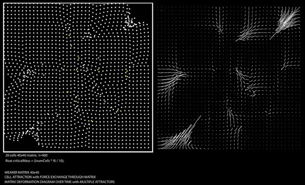
The Sabin & Jones architecture studio has examined the effects of branching morphogenesis in endothelial cells and how the attractive forces between the cells deform the substrate, which is modelled as an extra-cellular matrix, or ECM,

My own research into morphogenesis has revolved around the reaction-diffusion dynamics proposed by Alan Turing in the 50s. He was trying to find a mathematical model to explain pattern formation in organisms, from butterfly wing patterns to zebra stripes.

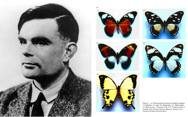
He proposed the diffusion of an activator and inhibitor through an evolving cellular system over a period of time, the concentration gradients dictating cell differentiation, ie a zebra skin cell can be black or white according to the concentration of a white-cell activator at the point when it forms. Biologists would call these activators morphogens, as these are the proteins that regulate gene expression. I’ve used these reaction-diffusion dynamics to explore morphology using generative graphics.

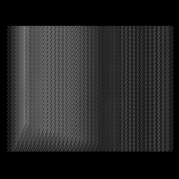
In my graphics I’ve used a growing matrix of straight lines, one added at each time step, to investigate what kind of formations this kind of dynamics can produce. My morphogens, an activator and inhibitor, hidden from view, are placed randomly on the canvas. They react, diffuse and deplete over time. In this graphic you can see a gradient operating from left-to-right, deforming lines and affecting line growth. No two vertical slices of this image are the same as a result. Gradients in morphogenesis are capable of creating this kind of heterogenous space, with no two spatial elements alike.

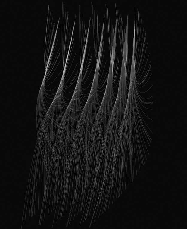
In this one you can see pattern formation in organic looking tendriled structures, lines curved out of shape by a force of attraction induced by the activator.

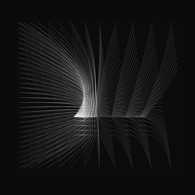
In this one you can see what happens when the inhibitor has a low concentration. Intensities appear around the location of the activator, which again acts as an attractor. Depending on the diffusion functions and reaction kinetics you choose and the property of your graphical components, there is a large phase space of potential morphologies. I’ve rendered many such parametric images as a means of visual thinking on the potential of morphogenetic dynamics to influence evolving urban form in a setting of decentralised urban policy.

In the urban analogy, you can think of these models as based on self-organising cells and a policy mechanism, in the form of a morphogen, that activates or inhibits certain cell behaviours. For example, you can think of planned retail or business locations as potential activators, activating residential ‘genes’ in cells as the concentration of the activator diffuses through space. Aura Reggiani of UCL has used reaction-diffusion dynamics to model how the cost of transportation influences population distribution in just such a manner. You can also think of the ECM as a street matrix, deformed by both attractors and cell interactions.

It should be noted that network representations of space, being discontinuous, can’t accurately express gradients. Information is invariably lost during the process of converting morphogenetically induced forms into networks.

Before moving on I’d like to briefly show you one more self-organising microscopic system, micelles,

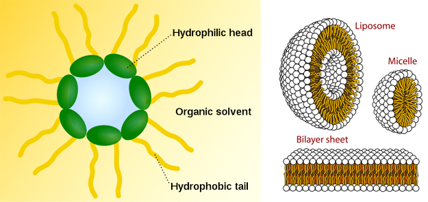
Sodium oleate molecules self-organise into a variety of forms, including spheres, circles and sheets, as a result of hydrophilic and hydrophobic molecular ends. Crucially though, this is just physics and chemistry acting on molecules — the system is not alive.

I want to skip to the urban scale now finally, to articulate some of my research aims. Looking at a multitude of complex systems has allowed me to properly situate my system of interest, namely the city. This 4-way chart show some of the complex systems I’ve looked at, situated on an axis of living to non-living and self-organised to organised. The term organised in this case referring to some form of centralised planning.

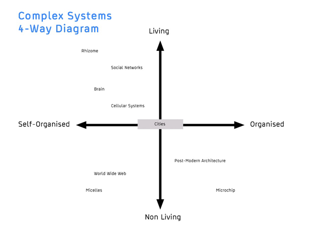
You can see microchips and post-modern architecture in the bottom right, brains, cellular systems and social networks in the top left, and micelles and the World Wide Web in the bottom left – these are non-living, self-organised complex systems. Cities however, fall squarely in the middle of these axes. They are living systems characterised by social interaction within a built environment and infrastructure. In part organised by central agencies, in part self-organising, in terms of all the unsupervised decisions made by individual developers. This organisational dynamic will vary depending on whether you’re looking at say, informal urbanism in the global south or the Western post-metropolis.

So, to my research aims.

One of my aims is to grow cities.

Growing Cities

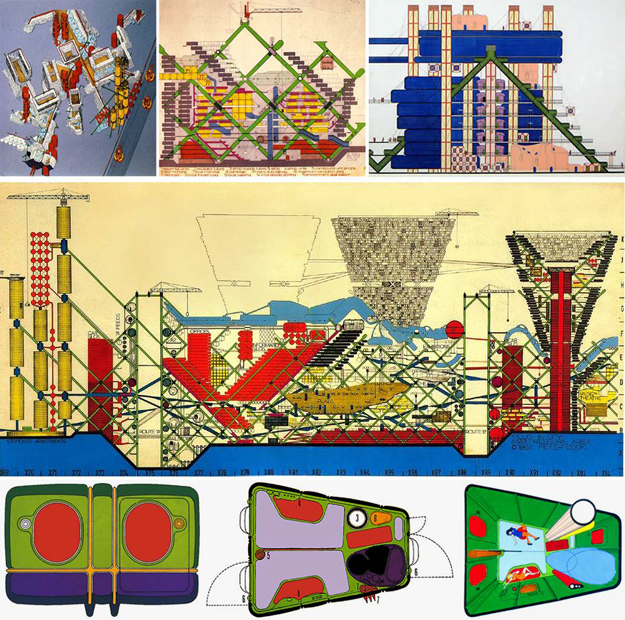
This tradition started out in architecture in the 60s, with the Bartlett’s own architectural group Archigram proposing this plug-in city, arranged within a huge scaffolding and presided over by a multitude of cranes. It was their assertion that organic, complex growth patterns could arise out of this adaptive framework of multi-storey, pluggable architectural units, that ‘organicness’ could arise out of heuristics.

The man with the cigar and the detachable collar in this image,

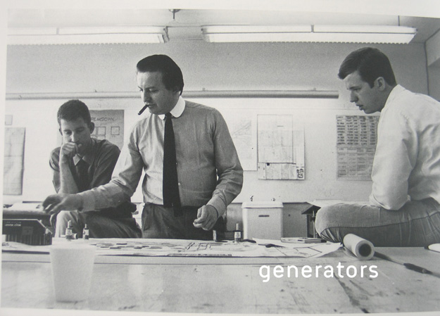
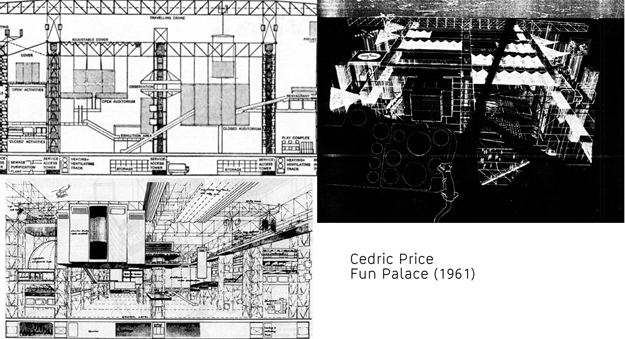
is Cedric Price. He introduced the term generator into architectural practice in the 60s, as part of his ideas relating feedback cybernetic systems to responsive architectures. These ideas went into his Fun Palace project, a proposed cultural center to be located on what is now London’s olympic site on the River Lea.

In my own research, I’m using Price’s term, generator, to describe a bottom-up urban policy ruleset designed to describe growth rules.

I’m conscious in this mode of enquiry of harking back to what Peter Hall has described as the heyday of systems planning, the 60s, which saw systems analysts propose many idealised forms for the city. Here are just four theoretical transport systems compiled in Haggert & Chortley’s excellent book from that era. Many of these are based on fairly reductive shortest path analysis.

A modern approach to urban growth models makes a significant departure, in that we are interested in growing emergent forms using bottom-up rulesets, or generators, which can be used to model environmental, transport or economic policy. In this cellular automata model by Bill Hillier in the 80s, he attempted to reproduce the complex form of French villages using placement rules for buildings.

My supervisor Mike Batty’s own research also contains a variety of growth models, including his work on the dual urban evolutionary model, or DUEM, designed as a predictive model for land use dynamics. Here are some of his attempts to model crystal growth systems with noise,

We can broadly categorise growth models into two types. First those that attempt to model aspects of real world urban systems. Secondly, a breed of growth model that attempts to incorporate development rulesets, or generators, to model new forms of economic, transport or environmental policy and analyse their results. One such algorithmic model is the complex grid, based on Mathieu Helie’s policy rulesets, which are designed to harness self-organisation.

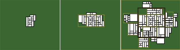
The three principles Helie states as the basis of his growth model are:

1. Any size of urban growth is allowed as long as the new growth extends the boundary of the network. This ensures that the city has the economic flexibility of the medieval city and allows anyone, no matter their economic importance, to contribute to the city’s growth.
2. The network must not become so complicated that it becomes impossible to move around in order to participate in large-scale activities and a culture of congestion.
3. Streets must not grow too long without interruption in such a way that speeding and traffic accidents are encouraged.

The rulesets allow private development on any available part of the network so long as the developer replace the part used up by extending the network around the new block. Community development can produce wider roads, which you can see in yellow.

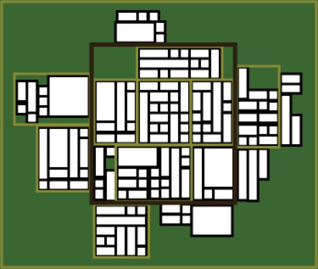
Policy interventions are allowed, only for the widening of existing links into ring roads that produce more of a small-world connectivity model.

Through this model Helie attempts to show how policy can reduce its predictive role in projecting growth through costly, speculative infrastructure investment, and reduce its organisational role in dictating precisely how growth occurs. The outcome, or so he claims, is sustainable growth based on dense urban form. It’s not without its complications however, as these kind of models are essentially behavioural models for planners and contain ideological statements about policy. They are also still simplistic.

But by building software models with these kind of growth rules, where policy acts like instructional DNA as opposed to the agent of a total, centralised vision, we can analyse how self-organisation can create urban environments with different connectivity properties to our contemporary cities and compare those differences.

One of my research aims is to produce algorithmic urban growth models which harness self-organisation by modeling growth according to these policy generators, investigating the resultant urban forms and providing an analytical toolkit to analyse the emergent morphologies. This will come in terms of a network analysis of their connectivity properties. These models will necessarily produce far more heterogenous form than the idealised forms produced by systems analysts in the 60s, as we begin to approximate morphogenetic dynamics through bottom-up rulesets.

My second research aim is a synthetic network analysis of London’s public transport systems, to include bus, rail and tube networks.

Urban Connectivity

Let’s look at scales of connectivity in the urban context as a means to understanding the basis of this work.

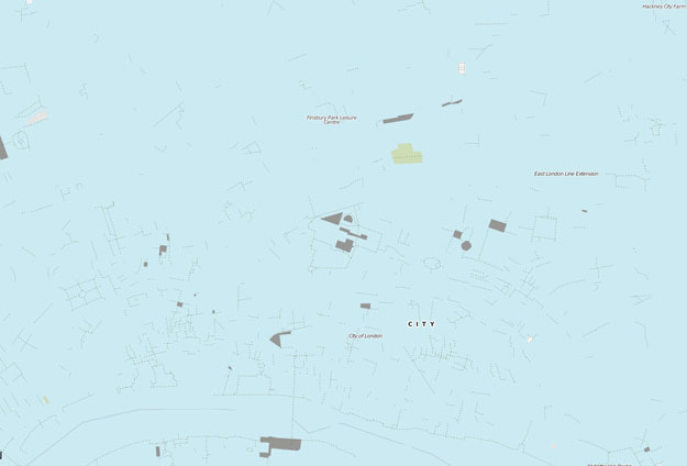
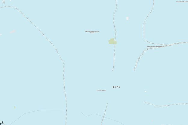
Here is a segment of East London, the northern tip of the City and Hoxton, about 3km wide. At the lowest end of our hierarchy of scales, we have the pedestrian network of footpaths represented as dashed lines. You can see it’s fragmented and incomplete. It’s reliant on networks further up the scale. We can say it’s poorly decoupled from other networks and not self-reliant. From a systems viewpoint, this strikes one immediately as poor design, as lower layers should generally not be dependent on upper layers in the system. Up the scale we have residential and tertiary roads,

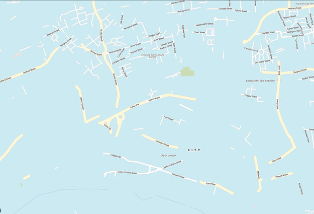
These too form archipelagos. You can see a single residential lattice up near the top but the rest is a set of incoherent fragments.

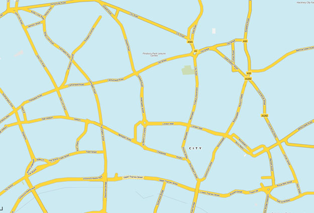
The primary and A-roads, by contrast, form a strong mesh of arteries. They have the most coherent form out of all the scales so far, identifiable as a single network. Finally we have the longer links of the underground system,

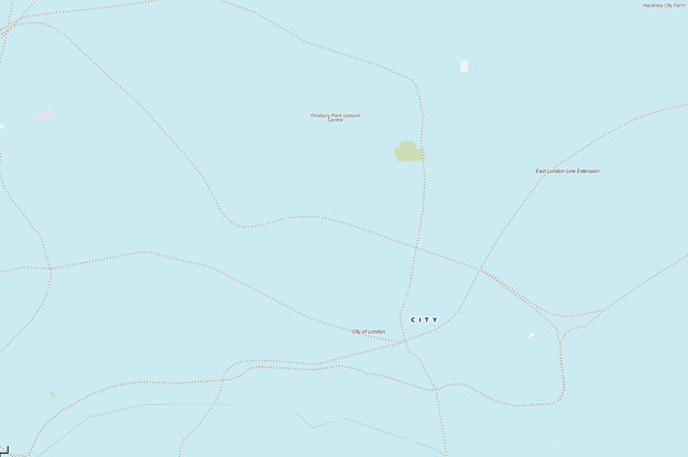
These links are obviously decoupled from all the others. And at the highest connectivity scale, we have long range railway links,

As we have seen, a diversity of scales of connectivity is a key property of self-organised complex systems. It helps them to deal with a multiplicity of transport scenarios. Scales of connectivity are also the basis for small-world properties in networks. My hypothesis is that a city can achieve this level of complexity through organised growth, and in doing so it can improve its efficiency in terms of the mobility of its inhabitants.

It’s part of my research aims to use an understanding of scales of connectivity and small-worlds to analyse representations of the public transport system in London, with a view to proposing interventions, in the form of link reconfiguration, deletion or addition, which improve global characteristic path lengths whilst retaining the high clustering properties that maximise movement potential at the neighbourhood scale.

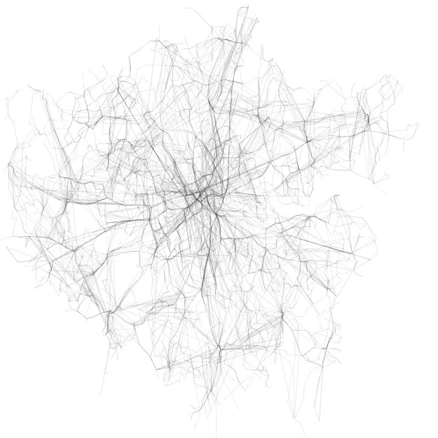
I’ve started with an analysis of the bus network. I’ll just show you some quick visualisations I’ve rendered for now. Here is London’s morphology as expressed through its 25,000 bus stops.

In this visualisation you can see the network representation of over 700 bus routes.

As I mentioned earlier, small interventions can tip a network from a poorly connected state to a small-world state, and in my analysis I’m trying to create techniques to spot where poor connectivity can be remedied with small interventions.

In this abstracted version,

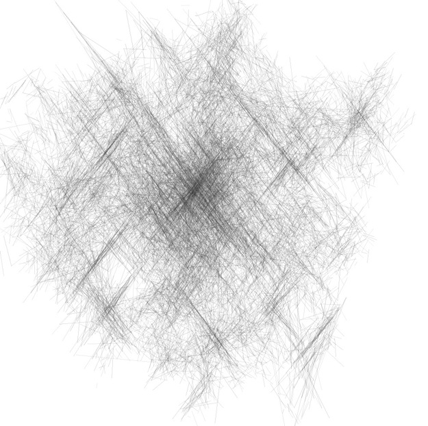
I’ve emphasised route directionality to get an idea of the intensity of routing in each direction. I have constrained links largely to horizontal, vertical or 45 degree angles, much as Harry Beck did in his classic London Underground map.

***

In summary, I’ve taken you through a diverse set of spatial systems to show you how network science can provide us with a vocabulary for comparative analysis.

I’ve shown how in self-organising complex systems of all sizes we can see efficiencies in terms of connectivity: we see scales of connectivity and small-world properties. These insights can provide us with models by which to quantify the well-formedness of urban transport networks. For example, I’ve touched on the brokenness of the pedestrian web in East London. There is scope for novel analysis and novel techniques for identifying low-cost reconfigurations of transport links based on these insights.

I’ve touched on how creating generative growth models for cities that embrace self-organisation through bottom-up policy rules, or generators, can provide insights into how to produce more sustainable urban form. Even our cursory glance at cell biology gives us clear examples of very dense yet decentralised spatial formations which allow for effective transport of nutrients through porous structures and boundary diffusion. These kind of insights into density, morphology and transport can contribute to the discourse on sustainable urban form and growth.

Lastly, I’ve introduced several concepts from morphogenetic systems, such as cells, gradients, extra-cellular matrix, motility and morphogens, which are useful when talking about emergent morphologies, a vocabulary that can be employed in the kind of urban growth models I am working with.

Thank you.

See Also: Network, Infrastructure, Cybernetics, Emergence, Morphogenesis, Space Syntax

Bibliography

• 1 Norbert Wiener, Cybernetics: or Control and Communication in the Animal and the Machine (Boston: The MIT Press, 1965)
• 2 Stanley Mathews, From Agit-prop to Free Space: The Architecture of Cedric Price (London: Black Dog Publishing, 2007)
• 3 Peter Cook et al, Archigram (New York: Princeton Architectural Press, 1999)
• 4 Chorley, R. J. and Haggett, P., Network Analysis in Geography (London: Hodder & Stoughton, 1969)
• 5 T. Sekimura, S. Noji, N. Ueno, P. K. Maini, Morphogenesis and Pattern Formation in Biological Systems (London: Springer, 2003)
• 6 Manuel Castells, Rise of The Network Society (Volume 1) (NJ: Wiley, 1996)
• 7 Bill Hillier, Julienne Hanson, The Social Logic of Space (Cambridge: Cambridge University Press, 1989)
• 8 Michael Batty, Cities & Complexity (Boston: MIT Press, 2007)
• 9 Nikos A. Salingaros, Principles of Urban Structure (Athens: Techne Press, 2005)
• 10 Gilles Deleuze, Felix Guattari, A Thousand Plateaus (London: Continuum, 2004)
• 11 Francesca Medda, Peter Nijkamp, Piet Rietveld, A Morphogenetic Perspective on Spatial Complexity (London: Springer, 2009)
• 12 Jamie A. Davies, Mechanisms of Morphogenesis (London: Elsevier, 2005)
• 13 Vojin G. Oklobdzija, Ram K. Krishnamurthy, High-Performance Energy-Efficient Microprocessor Design (Netherlands: Springer, 2006)
• 14 Peter Hall, Cities of Tomorrow: An Intellectual History of Urban Planning & Design in the Twentieth Century (New Jersey: Wiley-Blackwell, 2002)
• 15 Bocaletti et al, Complex networks: Structure and Dynamics Elsevier, Physics Reports 424 (2006) 175 – 308
• 16 Eguiluz et al, Scale-free brain functional networks, Physical Review Letters Vol. 94, 018102 (2005)
• 17 Sporns et al, Organization, development and function of complex brain networks , Elsevier, TRENDS in Cognitive Sciences Vol.8 No.9
• 18 Duncan J. Watts, Steven H. Strogatz, Collective Dynamics of Small World Networks, Nature, Vol. 393 (1998)
• 19 Steven H. Strogatz, Exploring complex networks, Nature Vol. 410 (2001)
• 20 M.Rosvall, C.T.Bergstrom, Maps of random walks on complex networks reveal community structure, PNAS Vol. 105 No. 4 (2008)
• 21 Michael Hensel, Achim Menges, Morpho-Ecologies: Towards Heterogeneous Space In Architecture Design (London: AA Publications, 2007)
• 22 Neil Leach, Digital Cities AD: Architectural Design (London: John Wiley & Sons, 2009)